LWD Tirol Meteo Download Package

Python package for downloading meteorological data of stations by the Avalanche Warning Service of Tyrol
python-package
data-download
Published

April 8, 2025

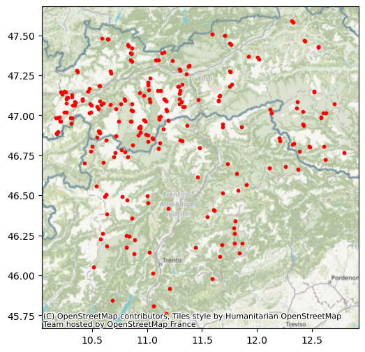
The package lwdmeteo is meant to facilitate download of meteorological data from the Avalanche Warning Service of Tyrol (Lawinenwarndienst Tirol, LWD Tirol). The package allows to retrieve a file (via get_station_file()) that contains all stations with some basic metadata which allows to explore when measurements start and what the corresponding station identifier (lwd-nummer) is. This station id must be passed to the actual download function (download_station(...) or batch_download_station(...)). A command line interface is also available with a description in the repository.

On the side of LWD Tirol, the files can be downloaded here for a specific station, variable and hydrological year. The lwdmeteo package simply sends requests to very same url that is accessed when downloading files via this page. Note that the data is licensed under CC BY 4.0.

Warning

The data available for download seems to be “raw” data and therefore should be carefully evaluated.

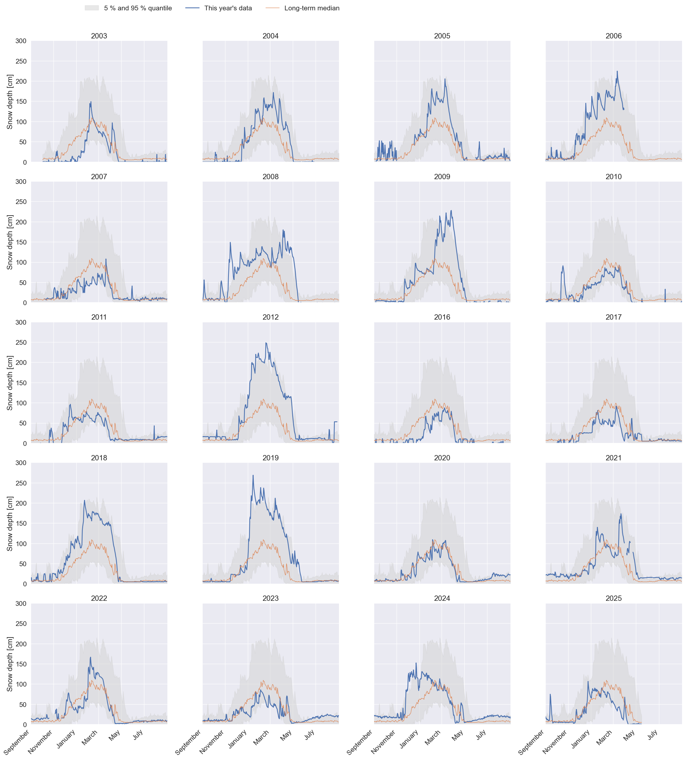
For the purpose of visualization, in the following I will use Sep. 1 as the start of the “hydrological” year, as I think it is a bit nicer since it captures snowfall events early in the season. Therefore I “define” the hydrological year in the following starting Sep. 1 which does not adhere to the actual definition.

Link to Gitlab Repo

import sys
import pandas as pd
import numpy as np
import seaborn as sns
import matplotlib as mpl
import matplotlib.pyplot as plt
import contextily as cx
import lwdmeteo
from lwdmeteo import batch_download_station, get_station_file, parameters

print(sys.version)
print(pd.__version__)
print(np.__version__)
print(sns.__version__)
print(mpl.__version__)
print(cx.__version__)
print(lwdmeteo.__version__)
3.13.1 | packaged by conda-forge | (main, Dec  5 2024, 21:23:54) [GCC 13.3.0]
2.2.3
2.2.0
0.13.2
3.10.1
1.6.2
0.1.0

Exploring available parameters

The keys of the dictionary are used to specify the desired parameter in the download function.

parameters
{'LT': 'Lufttemperatur',
 'LF': 'Luftfeuchte',
 'WG': 'Windgeschwindigkeit',
 'WR': 'Windrichtung',
 'GS': 'Globalstrahlung von oben',
 'HS': 'Schneehoehe',
 'T0': 'Oberflächentemperatur',
 'TP': 'Taupunkttemperatur',
 'WG.Boe': 'Windböe',
 'GS.unten': 'reflektierte Globalstrahlung'}

Exploring available stations

gdf_stations = get_station_file()
gdf_stations.head()
name operator lwd-nummer begin altitude geometry
0 Teufelsegg - Giovo del Diavolo Südtirol - Alto Adige STEU2 2007 3035.0 POINT (10.76466 46.7847)
1 Schaufeljoch LWD Tirol NSGS1 2012 3160.0 POINT (11.1109 46.9772)
2 Rossbänke - Pian dei Cavalli Südtirol - Alto Adige WROS2 2001 2255.0 POINT (10.81944 46.46935)
3 Lämmerbichlalm LWD Tirol TLAE2 1994 2020.0 POINT (11.75172 47.18127)
4 Niederthai Tiroler Wasserkraft AG UNIE2 1975 1564.0 POINT (10.96907 47.12284)

Visualization of station locations

Note that get_station_file() parses the response from here. This means that the following plot could look different if there are any updates in the future.

fig, ax = plt.subplots(figsize=(12, 6))

gdf_stations.plot(ax=ax, color="r", markersize=10)
cx.add_basemap(ax, crs=gdf_stations.crs)

plt.show()

Select station and retrieve measurement start

station = "LPUI2"  # Puitegg

gdf = get_station_file()
gdf.loc[gdf["lwd-nummer"] == station]
name operator lwd-nummer begin altitude geometry
203 Puitegg LWD Tirol LPUI2 2002 1539.0 POINT (11.15282 47.39484)

Let’s download the entire timeseries

parameter = "HS"  # snow depth

start_year = 2002
end_year = 2025

df = batch_download_station(station, parameter, start_year, end_year)

# resample to daily mean
df = df.resample("1D").mean()
# add hydrological year to df
df["hydro_year"] = df.index.to_series().dt.year + (df.index.to_series().dt.month >= 9)

Some (maybe overly complicated?) method to add the day-of-year starting september first

df["hydro_doy"] = df.index.to_series().dt.day_of_year
doy_values = np.copy(df.index.to_series().dt.day_of_year.values)

break_value = (
    244 + df.index.to_series().dt.is_leap_year
)  # DOY of Sep. 1 minus 1 day; in leap years Sep. 1
minus = break_value - 1
plus = 122  # nr of days after Sep. 1 - same every year

df.loc[doy_values >= break_value, "hydro_doy"] = (
    df.loc[doy_values >= break_value, "hydro_doy"] - minus
)
df.loc[doy_values < break_value, "hydro_doy"] = (
    df.loc[doy_values < break_value, "hydro_doy"] + plus
)

Clean up

  • Set values above 1 m snow depth in July and August to nan, as I assume these are measurement errors
  • Remove 2013, 2014 and 2015, it seems the data contains erroneous values in these years (not shown here)
cond = (
    (df.index.to_series().dt.month < 9)
    & (df.index.to_series().dt.month > 6)
    & (df["HS"] > 100)
)
df.loc[cond, "HS"] = np.nan

df = df.loc[~df["hydro_year"].isin([2013, 2014, 2015])]

Compute percentiles to be added to the plots as additional info (can be easily exchanged for min/max or other metrics)

Code
min_max = (
    df.groupby("hydro_doy")[["HS"]]
    .agg(
        min=("HS", lambda x: np.nanpercentile(x, 5)),
        max=("HS", lambda x: np.nanpercentile(x, 95)),
        med=("HS", lambda x: np.nanmedian(x)),
    )
    .reset_index()
)

Add upper and lower bounds of entire timeseries to original data frame for easier access

df_merged = df.reset_index().merge(min_max, on="hydro_doy").set_index("timestamp")
df_merged.head()
HS hydro_year hydro_doy min max med
timestamp
2002-10-03 0.000000 2003 33 -3.581250 19.069733 6.093536
2002-10-04 0.194444 2003 34 -2.737500 18.760327 5.895833
2002-10-05 0.305556 2003 35 -1.600694 18.482539 7.243056
2002-10-06 0.805556 2003 36 -2.391667 20.547516 8.152778
2002-10-07 0.847222 2003 37 -3.656250 21.091667 9.930556

Visualize

Titles specify the “hydrological year” starting Sep. 1.

Code
# generate ticklabels
dates_x = pd.date_range(start="2021-09-01", end="2022-08-31", freq="2MS")
ticklabels = dates_x.to_series().dt.strftime("%B").values
tickpos = dates_x.to_series().dt.day_of_year.values
dayvals = tickpos.copy()

tickpos[dayvals >= 244] = tickpos[dayvals >= 244] - 243
tickpos[dayvals < 244] = tickpos[dayvals < 244] + 122

sns.set_theme(font_scale=1.5)

g = sns.FacetGrid(
    df_merged,
    col="hydro_year",
    col_wrap=4,
    sharey=True,
    sharex=True,
    height=5,
    aspect=1.2,
)


def plot_with_minmax(data, color, **kwargs):
    plt.fill_between(
        data["hydro_doy"],
        data["min"],
        data["max"],
        color="lightgrey",
        label="5 % and 95 % quantile",
        alpha=0.5,
    )

    # use matplotlib directly, to avoid plotting NaN timesteps
    plt.plot(data["hydro_doy"], data["HS"], linewidth=2, label="This year's data")
    
    sns.lineplot(
        data=data, x="hydro_doy", y="med", linewidth=1, label="Long-term median"
    )
    plt.title(data["hydro_year"].iloc[0])


g.map_dataframe(plot_with_minmax)


def set_lim_label(color, xmin, xmax, ymax):
    ax = plt.gca()

    ax.set_xticks(tickpos, ticklabels, rotation=45, ha="right")

    ax.set_xlim((xmin, xmax))
    ax.set_ylim((0, ymax))
    ax.set_ylabel("Snow depth [cm]")
    ax.set_xlabel(None)


g.map(set_lim_label, xmin=1, xmax=366, ymax=300)

g.add_legend(loc="lower left", bbox_to_anchor=(0.1, 1.01), ncol=3)

plt.savefig(f"{station}-snow-depth.png", dpi=100, bbox_inches="tight")
plt.show()